The Numbers Behind Trade

Would you rather have €100 today or €115 in one year? The answer is mathematics. A joint seminar by the Math Society and IB&CM Society — from the time value of money to Black–Scholes.

Meet the Speakers

Eyosiyas

Contributed to the seminar with insights into financial applications and helped connect the mathematical theory to real-world trading and market behaviour.

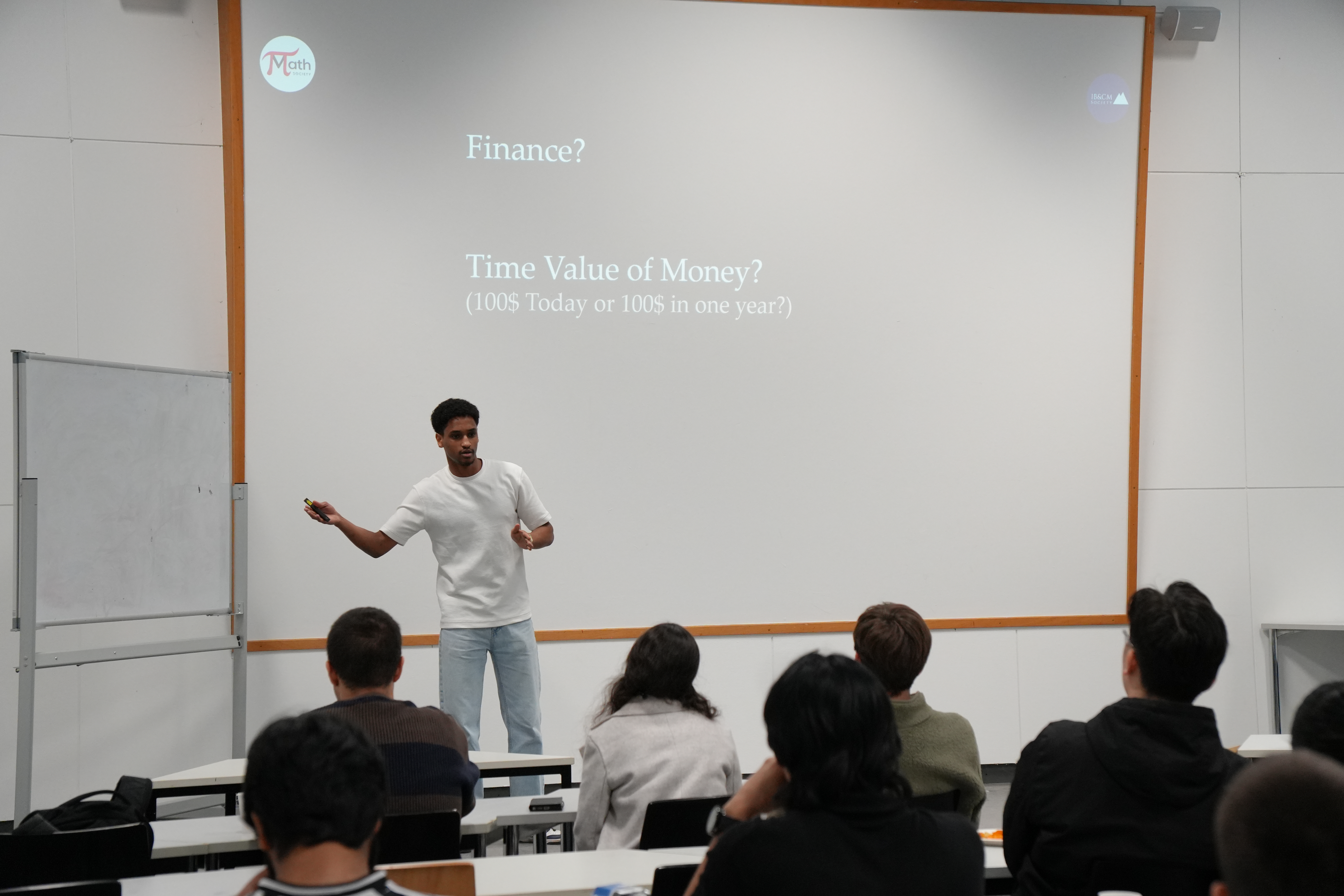
"€100 today or €100 in one year?"

Ahmed

Formalised no-arbitrage theory, derived European call pricing via replicating portfolios and binomial trees, then built up to Brownian motion and the Black–Scholes PDE.

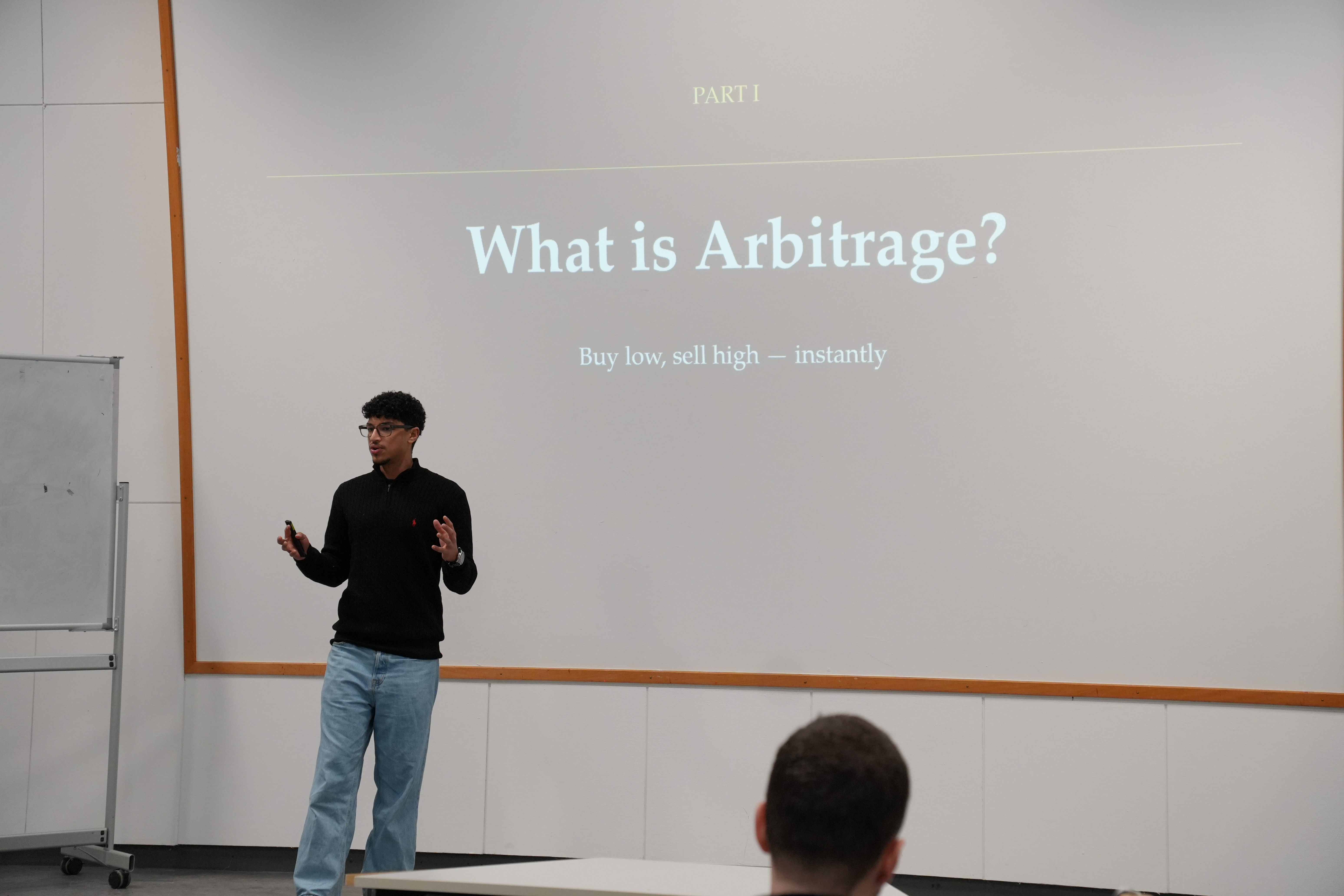
"Buy low, sell high — instantly"

Muhammad

Contextualised it all through quantitative finance — who quants are, where they work, and how HFT strategies exploit market inefficiencies in milliseconds.

"Math → Finance?"

💰

Time Value of Money & Portfolios

A euro today is worth more than a euro tomorrow — inflation erodes purchasing power over time. This gives us present value and future value: tools to compare money across time. If €100 grows to €105 at 5% interest, then the present value of €105 in one year is €100.

Why not just save? Real savings returns rarely beat inflation. The rational move is to invest across a portfolio of stocks, bonds, and commodities — spreading risk so no single failure wipes you out.

⚖️

Arbitrage & The Law of One Price

Arbitrage exploits price differences for the same asset in different markets for a risk-free profit. Arbitrageurs self-correct free markets, enforcing the law of one price: identical assets must trade at the same price everywhere.

          Triangular forex example: €1 → $1.20 → £0.96 → €1.056. A 5.6% gain by cycling through three
          momentarily inconsistent exchange rates.
        

No-Arbitrage Assumption

Formally: a portfolio h is an arbitrage iff its cost today is ≤ 0 while its payoff is ≥ 0 in every state (strictly positive in at least one). The no-arbitrage assumption asserts no such h exists — not because it never appears, but because HFT exploits it so fast it vanishes instantly.

H is an arbitrage ⟺ p·h ≤ 0 and A·h ≥ 0 (strictly positive in at least one state)

🛡️

Hedging & Options

Hedging is financial insurance — holding an asset that rises when your main investment falls. Options are the primary tool: you pay a premium upfront for the right (not obligation) to buy or sell at a fixed price.

📞 Call Option

Right to buy at strike price K. Valuable when you expect the price to rise.

📤 Put Option

Right to sell at strike price K. Valuable when you expect the price to fall.

💎 Strike Price (K)

The fixed price at which the holder may buy or sell.

🏷️ Premium

The upfront cost of the option — paid regardless of whether it's exercised.

          Example: You hold stock at $100 and buy a put at K = $100. If it drops to $70, the put pays
          $30 — offsetting your loss. If it rises to $120, let the option expire and keep the gain. Unlimited upside,
          capped downside.
        

🧮

Pricing Options: The Binomial Tree

To price a European call, we find a replicating portfolio of Δ shares and B bonds matching the option's payoff in each outcome. By the law of one price, the option must cost exactly Δ·S + B today. This simplifies to a risk-neutral probability q = (y − d) / (u − d):

C = q · C_U + (1 − q) · C_D · (discount factor)

q is not the real probability of the market going up — it's a synthetic measure under which the expected stock payoff equals its price today. Extending to multiple periods (the binomial tree) gives the general closed form:

C = e^−nr · Σ_j=0ⁿ C(n,j) · q^j · (1−q)^n−j · max(0, S·u^j·d^n−j − K)

🔬

Quantitative Finance & The World of Quants

Quants are the mathematicians at the heart of modern finance. They work across three types of institutions:

Investment Banks (e.g. Deutsche Bank): price and sell derivatives.

Hedge Funds & Trading Firms (e.g. Renaissance Technologies): build proprietary models to generate returns.

Asset Managers (e.g. pension funds): manage large portfolios and control risk.

Their work: price instruments, manage risk, and build trading strategies — automated programs that exploit statistical patterns across millions of trades per day, often in under a second.

📐

Brownian Motion & Black–Scholes

Real markets move continuously, not in discrete steps. Stock prices follow geometric Brownian motion — always positive, driven by a random Wiener process W(t):

S(t) = S(0) · exp( (μ − σ²/2)t + σ·W(t) )

Because dW² = dt (variance grows linearly in time), the classical chain rule breaks. Itô's lemma corrects this with an extra term:

df = f'(W) dW + ½ f''(W) dt

Applying Itô's lemma to C(S,t), constructing a delta-hedged replicating portfolio, and invoking no-arbitrage yields the Black–Scholes PDE:

∂C/∂t + ½ σ² S² · ∂²C/∂S² + r·S · ∂C/∂S − r·C = 0

Solving with boundary condition C(S,T) = max(S − K, 0) gives the Black–Scholes formula — the mathematical engine behind the multi-trillion dollar derivatives market.

Key Takeaways:

€1 today > €1 tomorrow — always invest, never just save.
Arbitrage enforces the law of one price across all free markets.
Options give unlimited upside with capped downside.
Risk-neutral pricing: discount the expected payoff under a synthetic probability measure.
Stock prices follow geometric Brownian motion — always positive and continuous.
Because dW² = dt, classical calculus fails; Itô's lemma provides the fix.
Black–Scholes PDE: the equation whose solution prices any European option.

Finance looks like intuition. Underneath, it is mathematics — all the way down to the partial differential equation.