Correlation is not causation — you've probably heard this before. But what does it actually mean for machines that learn from data? And how do we teach a model not just what happened, but why?
At this event, two of our own members — Eyosiyas and Idamis — took us on a journey from basic probability all the way to causal inference, showing how going beyond correlation unlocks a fundamentally more powerful kind of machine learning.
Meet the Speakers

Eyosiyas
Second-year IEM student, originally from Ethiopia — and also the Math Society's Logistics & Project Management Lead. He walked us through the mathematical backbone of causal reasoning: random variables, DAGs, d-separation, and structural causal models.
Idamis
First-year Industrial Engineering student from the Dominican Republic. Idamis brought causal theory to life through the lens of correlation vs. causation, Pearson coefficients, interventions, and the do-operator — drawing the contrast with traditional machine learning throughout.

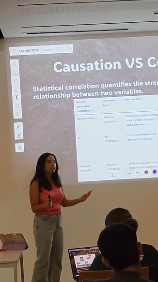
Eyosiyas and Idamis taking the audience through the session together
Starting From Scratch: Probability & Random Variables
The talk opened with the question: why do we even need probability? Because the future is uncertain. We can never know exactly how many orders will come in next month, or whether a customer will stay. But we can describe uncertainty mathematically — and that's where random variables come in.
A random variable converts a qualitative outcome into a number. Flip a coin: heads becomes 1, tails becomes 0. There are two flavours:
Continuous random variables — measurable outcomes. Delivery time can be 1 day and 10 hours — any real value on the number line.
The running example for the entire talk: an e-commerce company trying to understand whether delivery time affects customer retention. Simple enough to follow. Deep enough to reveal all the traps of naive data analysis.
Joint & Conditional Probability
Joint probability captures two things happening at once — for example, a customer receiving fast delivery and staying with the company. Conditional probability zooms in: given that delivery was fast, what's the chance the customer stayed? If 80% of fast-delivery customers retained, that conditional probability is 0.8.
Two variables are independent when knowing one gives you no extra information about the other — mathematically, when P(X) × P(Y) = P(X, Y). In our example, delivery speed and retention are dependent: changing the delivery time does shift how likely customers are to stay.
Correlation vs. Causation: Why It Matters
Ice cream sales and drowning rates both rise in summer — they are correlated. But ice cream doesn't cause drowning; hot weather causes both. This is the classic trap of correlation without causation, and it's exactly the trap that traditional machine learning falls into.
Correlation: two variables move together — but the movement might be caused by a hidden third factor, pure coincidence, or a genuine causal link. Correlation alone can't tell you which.
To measure correlation numerically, we use the Pearson correlation coefficient. It ranges from −1 to +1: a value near +1 means the variables rise together, near −1 means one rises as the other falls, and 0 means no linear relationship. But crucially — a non-zero Pearson coefficient tells you nothing about why those variables are related.
A graph of on-time delivery rate versus customer satisfaction shows a clear negative correlation: longer delays, lower satisfaction. A traditional ML model sees this pattern and learns from it. But it has no idea what is causing what — and that ignorance matters the moment you want to intervene.
Directed Acyclic Graphs (DAGs): Drawing Causality
Enter the Directed Acyclic Graph — a tool for making causal assumptions explicit. Each variable becomes a node. An arrow from X to Y means "X causes Y." Two rules define a valid DAG:
Acyclic: you cannot follow the arrows and end up back where you started. No variable can be its own cause.
In the delivery example, customer income is a confounder — it influences both delivery speed (richer customers may pay for faster delivery) and retention (wealthier customers may be more loyal regardless). Ignore it, and you'll wrongly attribute the entire retention effect to delivery time alone.
Confounders and Colliders
Two structural patterns are essential to recognize in any DAG:
Collider: a variable Z with arrows pointing in from both X and Y. Conditioning on a collider (or its descendants) actually opens a path between X and Y that was previously blocked — the opposite of what you might expect.
The cat-and-lamp example from the talk illustrated this beautifully. You observe that on 10 out of 100 days your cat was inside, the lamp was on the floor. Suspicious. But those same 10 days there was an earthquake. The earthquake is a confounder: it drove the cat indoors and knocked the lamp over. To test whether the cat is truly to blame, you need to force the cat inside on days when there is no earthquake — that's an intervention.
D-Separation: When Are Two Variables Independent?
D-separation is the graphical rule for reading conditional independence directly off a DAG — no calculations needed. It relies on three rules:
Rule 2: A path is blocked if it contains a collider and neither that collider nor any of its descendants has been conditioned on.
Rule 3: Conditioning on a collider (or a descendant of a collider) unblocks the path — the collider no longer acts as a barrier.
Two variables are d-separated if every path between them is blocked. D-separated variables are conditionally independent. In practice, this lets you figure out which variables you need to control for in order to isolate a genuine causal effect — and which ones you should not condition on (namely, colliders).
Interventions & The Do-Operator
There is a fundamental difference between observing that your phone is on the floor after it fell, and throwing the phone on the floor yourself. Both result in the same event — but one is observation, the other is an intervention. Causal machine learning is built on this distinction.
Formally, we write interventions using the do-operator. Instead of asking "what is the probability of Y given that X equals x?" — which is merely observational — we ask:
This asks: if we force X to take the value x — cutting all its incoming arrows in the DAG — what happens to Y? The do-operator is what allows causal models to answer "what if" questions, not just describe past patterns.
Structural Causal Models (SCMs)
A Structural Causal Model brings together a DAG and a set of equations describing how each variable is generated. It distinguishes between endogenous variables — the ones you can observe and model directly (delivery time, customer retention) — and exogenous variables, the unmeasured noise that affects outcomes in ways you cannot fully control (a customer's mood that day, an unexpected road closure).
Working with an SCM involves three steps: abduction (observe the data), action (apply the do-operator to simulate an intervention), and prediction (compute the downstream effect). These three steps mirror the scientific method — and they are what make causal ML genuinely capable of answering questions that traditional ML cannot.
Identifiability & The Back-Door Criterion
Even with a DAG, we still need to know: can we actually estimate the causal effect from the data we have? This question is called identifiability. If confounders are creating back-door paths from the treatment variable to the outcome, we need to block those paths before we can trust our estimate.
The back-door criterion gives us a recipe: find a set of variables Z such that conditioning on Z blocks all back-door paths from X to Y (without opening any collider paths). Once that condition is met, the causal effect becomes identifiable using the adjustment formula:
Applied to the delivery example: if we want to know the true effect of one-day delivery on retention, we condition on customer income group (the confounder), compute the retention rate separately for each income group, then take a weighted average. With income-group probabilities of 0.6 (high) and 0.4 (low), and observed retention rates of 90% and 70% respectively, the causal estimate comes out at 0.9 × 0.6 + 0.7 × 0.4 = 0.82 — an 82% retention probability under forced one-day delivery, cleaned of any confounding from customer income.
Traditional vs. Causal Machine Learning
With everything in place, here is how the two paradigms compare:
| Dimension | Traditional ML | Causal ML |
|---|---|---|
| Core question | How are variables correlated? | What causes what? |
| Uses DAGs? | No | Yes — central to the approach |
| Interventions | Not modelled | Explicit via the do-operator |
| Counterfactuals | Cannot answer "what if?" | Answered through SCMs |
| Confounders | May absorb without noticing | Blocked explicitly via back-door adjustment |
| What it learns | Patterns in the surface statistics | The underlying data-generating mechanism |
- Probability quantifies uncertainty; random variables make it computable
- Correlation measures association — it says nothing about the direction or source of a relationship
- DAGs make causal assumptions explicit and auditable
- D-separation lets you read conditional independence directly from the graph
- The do-operator distinguishes observation from intervention — the heart of causal ML
- The back-door criterion identifies which variables to control for when estimating causal effects
- Causal ML can answer "what if?" — traditional ML cannot
Machines that only see patterns will always be fooled by coincidence. Machines that understand cause and effect can change the world.